Vector clustering of search queries: build your own system with ChromaDB, embeddings, and Python

Would you like to try Octo Browser at а discount?
Use the promo code OCTOBLOG to get 30% off any subscription. This offer is valid only for new users.

Collecting semantic data

There are several approaches to collecting semantic data, but the basic process is usually built around the same pattern: first, an initial pool of queries is created using services such as Google Ads Keyword Planner and other tools that provide search-volume data for the relevant topic.

The initial set is then expanded with related queries, search suggestions, and additional semantic sources. Key Collector was often used for similar tasks in the past, but today it is often necessary to combine several tools or use custom scripts to collect the necessary data.

Using automation tools to collect semantic data

If commercial solutions don’t fit your budget, functionality requirements, or limitations, you can automate part of the semantic collection process yourself. For example, to retrieve search suggestions and other data from web interfaces, you can use headless browsers based on Puppeteer or Playwright.

If you’re collecting semantic data across a large number of parallel sessions, you need to manage browser profiles and their environments safely. Here you can use an anti-detect browser such as Octo Browser to isolate sessions, manage profile settings, and connect different proxies. This simplifies the scraping infrastructure and reduces the amount of manual configuration required for each individual browser instance.

The main challenge when collecting data at scale is the restrictions imposed by search engines. Automated requests may trigger rate limits, CAPTCHAs, or other protection mechanisms, so when designing such a pipeline, you need to account for session stability, request frequency, and temporary blocks.

When working with browser automation, it is also important to control environment parameters such as the User-Agent, window size, locale, WebGL, and other browser-session characteristics. You can do this using your own Puppeteer or Playwright configurations or specialized browser solutions that let you create isolated profiles with different environment parameters.

Another separate task is organizing the network infrastructure. You can use different types of proxies for distributed data collection: datacenter, residential, or mobile. The choice depends on request volume and requirements for stability, speed, and cost. Datacenter proxies are usually cheaper and faster, but in certain scenarios they are more likely to be restricted. Residential and mobile addresses are generally more resilient, but they cost more and offer lower throughput.

Once the main data collection is complete, you can supplement the final list of queries with data from external semantic databases. The result should be as complete a set of queries as possible, which can then be passed to the cleaning, normalization, and further clustering stages.

Cleaning data before vectorization

After collecting your semantic data, you will have a file containing tens of thousands of search queries. At first glance, it may seem ready for vectorization and clustering, but the quality of the result depends heavily on how well the data is prepared beforehand.

At this stage, the Pandas and NumPy libraries are convenient for cleaning and normalizing the input dataset. A raw query list almost always contains duplicates, unnecessary characters, technical clutter, irrelevant phrases, and other artifacts introduced during parsing and the merging of multiple sources.

An embedding model will convert these strings into vectors anyway, but this creates unnecessary computational overhead and may degrade the structure of the resulting clusters. That is why it is a good idea to bring the data into a consistent and predictable format before vectorization.

The main preparation stages are as follows:

• Removing technical clutter. HTML tags, extra spaces, invisible characters, emojis, and other elements that may have entered the data during scraping are removed.

• Global deduplication. When combining queries from multiple sources, overlaps are almost inevitable. There is no point in vectorizing identical strings more than once, so complete duplicates should be removed in advance.

• Stop-word filtering. At this stage, you can exclude queries containing irrelevant place names, unwanted markers, or words that do not fit the project requirements. For example, commercial semantic data may exclude queries with words such as “free,” “torrent,” and similar modifiers.

• Reducing words to their dictionary form (lemmatization) is optional. Modern models understand different forms of the same word and equivalent phrases well. For example, they can recognize that “buy iPhone” and “I want to buy an iPhone” are almost the same query. So there is no need to deliberately change words before processing. However, simple preprocessing can help identify similar queries and reduce the amount of data.

The result should be a clean and filtered set of unique queries without obvious technical noise. The data can then be passed to the next stage—converting text into vector representations.

Vectorizing search queries

Vector clustering differs from traditional string comparison because it works not with exact word matches, but with their semantic representations. Each search query is converted into a numerical vector—an embedding—that encodes its semantic characteristics.

Specialized embedding models are used for this. The text is first split into tokens, after which the model generates a vector of a fixed dimensionality. As a result, semantically similar queries are positioned closer to each other in vector space.

For example, the phrases “buy iPhone 15” and “iPhone 15 Pro price” will have more similar vectors than “buy iPhone 15” and “Apple phone repair.” This property makes it possible to use clustering algorithms to group queries.

Commercial solutions (OpenAI, Claude)

For vectorization, you can use both cloud APIs and local models. The choice depends on the amount of data, quality requirements, available infrastructure, and the acceptable processing cost.

Commercial APIs are convenient because they do not require local model deployment and let you get started quickly. The provider takes care of the infrastructure, model updates, and computational scaling.

For small and medium-sized datasets, this is one of the simplest solutions. However, when processing hundreds of thousands or millions of queries, you need to consider API costs, request limits, and throughput.

In addition, working with APIs requires a fault-tolerant architecture (bypassing API limits by multi-accounting, key rotation, and asynchronous requests via aiohttp).

You can test how commercial neural networks work with your queries yourself using the following code:

import os
from openai import OpenAI

# Initialize the client
client_ai = OpenAI(api_key=os.environ.get("OPENAI_API_KEY"))

# Our raw dataset
queries = ["buy iphone 15", "iphone 15 pro price", "apple phone repair"]

# 1. Vectorize queries through OpenAI
response = client_ai.embeddings.create(
    input=queries,
    model="text-embedding-3-small"
)

# The result is a set of ready-made multidimensional vectors
embeddings = [data.embedding for data in response.data]

import os
from openai import OpenAI

# Initialize the client
client_ai = OpenAI(api_key=os.environ.get("OPENAI_API_KEY"))

# Our raw dataset
queries = ["buy iphone 15", "iphone 15 pro price", "apple phone repair"]

# 1. Vectorize queries through OpenAI
response = client_ai.embeddings.create(
    input=queries,
    model="text-embedding-3-small"
)

# The result is a set of ready-made multidimensional vectors
embeddings = [data.embedding for data in response.data]

Local models from the Hugging Face ecosystem

An alternative to commercial APIs is open embedding models that run locally. For example, for multilingual tasks, you can use jinaai/jina-embeddings-v3 or Alibaba-NLP/gte-multilingual-large, which do not incur per-generation costs.

from sentence_transformers import SentenceTransformer

print("⏳ 1. Loading stable BGE-m3 model...")
model = SentenceTransformer('BAAI/bge-m3')

queries = ["buy iphone 15", "iphone 15 pro price", "apple phone repair"]

print(f"⏳ 2. Vectorizing {len(queries)} queries...")
embeddings = model.encode(queries, normalize_embeddings=True)

print("\n✅ Done! Let's look at the result:")
print(f"📊 Data dimensions: {embeddings.shape}")
print("🔍 Vector for the phrase 'buy iphone 15':")
vector_preview = [round(float(num), 4) for num in embeddings[0][:5]]
print(f"🔢 {vector_preview} ... and {len(embeddings[0]) - 5} more numbers.")

from sentence_transformers import SentenceTransformer

print("⏳ 1. Loading stable BGE-m3 model...")
model = SentenceTransformer('BAAI/bge-m3')

queries = ["buy iphone 15", "iphone 15 pro price", "apple phone repair"]

print(f"⏳ 2. Vectorizing {len(queries)} queries...")
embeddings = model.encode(queries, normalize_embeddings=True)

print("\n✅ Done! Let's look at the result:")
print(f"📊 Data dimensions: {embeddings.shape}")
print("🔍 Vector for the phrase 'buy iphone 15':")
vector_preview = [round(float(num), 4) for num in embeddings[0][:5]]
print(f"🔢 {vector_preview} ... and {len(embeddings[0]) - 5} more numbers.")

The main advantage of local models is that the entire processing pipeline remains within your own infrastructure. You process search queries without sending them to a third-party API, and once the model is loaded, you can vectorize them without paying for each individual request.

Working with local models is often more cost-effective: they let you perform vectorization without paying for every API call. At the same time, they require a significant amount of disk space: together with model weights and cache, they can take up several gigabytes. If you no longer need a model, it is a good idea to remove its local files and clear the cache after you finish working with it.

Storing and searching vector representations

After vectorization, each search query is represented as an embedding vector. The next question is where to store this data and how to efficiently find semantically similar queries.

For small datasets, vectors can remain in memory, for example in NumPy arrays or Pandas structures. If there are only a few thousand queries, this is usually enough for experiments and local processing.

As the dataset grows, the situation changes. If every vector is compared directly with all the others, the number of operations grows quadratically. For tens or hundreds of thousands of queries, this quickly becomes resource-intensive in terms of both computation time and memory usage.

This problem is solved with vector databases. They are optimized specifically for such tasks and support approximate nearest-neighbor search algorithms (in particular, HNSW). Built-in indexes make it possible to avoid directly comparing every vector with every other vector and provide almost instant searches for the most similar phrases even among millions of records.

There are several popular solutions for these tasks: Pinecone, Qdrant, PostgreSQL with the pgvector extension, and others. In our example, we will use ChromaDB. It is well suited for local experiments: it runs without a separate server, stores data on disk, and integrates easily with Python code.

Let’s save the embeddings obtained at the previous stage and check how semantic search works:

import chromadb

# 1. Initialize the local database (creates the semantic_db folder)
client = chromadb.PersistentClient(path="./semantic_db")

# 2. Create the collection
collection = client.get_or_create_collection(
    name="search_queries",
    metadata={"hnsw:space": "cosine"}
)

# 3. Load our vectors and query texts
collection.add(
    embeddings=embeddings.tolist(), # vectors from our local BGE-m3 model
    documents=queries,
    ids=["id_1", "id_2", "id_3"]
)
print("✅ Data saved to the database!\n")

# ==========================================
# SEARCH MAGIC: let's check how the database understands meaning
# ==========================================
test_phrase = "how much does the new iphone cost"
print(f"Searching the database for the phrase: '{test_phrase}'")

# Convert the test phrase into a vector using the same model
test_embedding = model.encode([test_phrase], normalize_embeddings=True)

# Ask the database to find the two most similar options
results = collection.query(
    query_embeddings=test_embedding.tolist(),
    n_results=2
)

print(f"Closest query: {results['documents'][0][0]} (Distance: {results['distances'][0][0]:.4f})")
print(f"Second closest: {results['documents'][0][1]} (Distance: {results['distances'][0][1]:.4f})")

import chromadb

# 1. Initialize the local database (creates the semantic_db folder)
client = chromadb.PersistentClient(path="./semantic_db")

# 2. Create the collection
collection = client.get_or_create_collection(
    name="search_queries",
    metadata={"hnsw:space": "cosine"}
)

# 3. Load our vectors and query texts
collection.add(
    embeddings=embeddings.tolist(), # vectors from our local BGE-m3 model
    documents=queries,
    ids=["id_1", "id_2", "id_3"]
)
print("✅ Data saved to the database!\n")

# ==========================================
# SEARCH MAGIC: let's check how the database understands meaning
# ==========================================
test_phrase = "how much does the new iphone cost"
print(f"Searching the database for the phrase: '{test_phrase}'")

# Convert the test phrase into a vector using the same model
test_embedding = model.encode([test_phrase], normalize_embeddings=True)

# Ask the database to find the two most similar options
results = collection.query(
    query_embeddings=test_embedding.tolist(),
    n_results=2
)

print(f"Closest query: {results['documents'][0][0]} (Distance: {results['distances'][0][0]:.4f})")
print(f"Second closest: {results['documents'][0][1]} (Distance: {results['distances'][0][1]:.4f})")

Choosing a clustering algorithm

Once the embedding vectors have been obtained, you can move on to the next stage—grouping search queries. At this stage, it is important to choose an algorithm that matches the structure of the data and does not require overly rigid assumptions about the number of future clusters.

Why K-Means is not always suitable for SEO clustering

K-Means is a classic clustering algorithm that divides data into a predefined number of groups. The number of clusters is specified with the k parameter.

For example, if we have 10,000 search queries and specify k=500, the algorithm will create 500 centroids and assign each query to the nearest one in vector space.

The main limitation of this approach is that the number of clusters must be determined in advance. This is not always convenient for a semantic core: before processing begins, it is difficult to know how many independent intent groups the dataset contains—50, 500, or 1,200.

If k is chosen poorly, related queries may end up split across several groups. The reverse can also happen: queries that are close in topic but differ in intent may be merged simply because the algorithm has to create the specified number of clusters.

Clustering with DBSCAN

If the number of groups is not known in advance, you can use density-based clustering algorithms. One of the best-known solutions is DBSCAN (Density-Based Spatial Clustering of Applications with Noise).

Unlike K-Means, DBSCAN does not require you to specify the number of clusters beforehand. The algorithm searches for regions in vector space where objects are sufficiently close together and forms groups from them.

DBSCAN behavior is determined by two main parameters:

1. eps (epsilon/distance): the maximum distance between points at which they are considered neighbors. In our case, this is the cosine-similarity threshold of the vectors.

2. min_samples: the minimum number of neighbors required to form a full cluster.

DBSCAN takes the first random query. If there are min_samples other queries within an eps radius of it, a cluster core is formed. The algorithm then expands in all directions, adding new neighbors until the density runs out.

The eps parameter can roughly be compared to the strictness of clustering:

• A smaller eps corresponds to stricter grouping. Only queries with very similar vector representations will end up in the same cluster, so you usually get more groups, and they become more compact.

• A larger eps makes the merging conditions more permissive. Clusters become larger and may include broader semantics, but the risk of combining queries with different intents also increases.

Another useful property of DBSCAN is its ability to identify noise. If a query is not located in a sufficiently dense region of vector space, the algorithm does not try to force it into one of the existing clusters. Instead, it marks the query as an Outlier. You can export these queries to a separate file for manual review instead of compromising otherwise clean landing pages.

At the same time, DBSCAN is sensitive to the choice of eps: a single threshold does not always work well with data in which some groups are very dense and others are much more sparse.

In such cases, consider HDBSCAN, a hierarchical extension of the density-based approach. It can find clusters with different densities, automatically adapting the eps parameter where queries are more tightly packed or, conversely, more dispersed.

The clustering script

Let’s extract our vectors from the local ChromaDB database and run them through DBSCAN using the scikit-learn library:

import chromadb
import numpy as np
from sklearn.cluster import DBSCAN

print("⏳ 1. Connecting to the vector database...")
client = chromadb.PersistentClient(path="./semantic_db")

# Extract the collection with the vectors (use your own name)
collection = client.get_collection(name="search_queries") 

# Extract all query texts and their mathematical vectors
data = collection.get(include=["documents", "embeddings"])
documents = data["documents"]
embeddings = np.array(data["embeddings"])

print(f"✅ Queries extracted from the database: {len(documents)}")

# ==========================================
# CLUSTERING (DBSCAN)
# ==========================================
print("⏳ 2. Starting the DBSCAN algorithm...")

# SETTINGS:
# eps = 0.15 (Allowed cosine distance. The smaller it is, the stricter the clusters);
# min_samples = 2 (Minimum of 2 queries to create a group);
# metric="cosine" (We explicitly specify that we measure angles between vectors, not linear distance).
dbscan = DBSCAN(eps=0.15, min_samples=2, metric="cosine")

# Run the grouping
labels = dbscan.fit_predict(embeddings)

# ==========================================
# OUTPUT RESULTS
# ==========================================
# The algorithm assigned each query a group number (0, 1, 2...). 
# If a query is recognized as noise (Outlier), it receives the label -1.

clusters = {}
outliers = []

for doc, label in zip(documents, labels):
    if label == -1:
        outliers.append(doc)
    else:
        if label not in clusters:
            clusters[label] = []
        clusters[label].append(doc)

print("=== GROUPING RESULTS ===")
for cluster_id, docs in clusters.items():
    print(f"\n Cluster #{cluster_id} (Queries: {len(docs)})")
    for d in docs:
        print(f"  - {d}")

if outliers:
    print(f"\n Outliers/Noise (Queries: {len(outliers)})")
    for out in outliers:
        print(f"  - {out}")

import chromadb
import numpy as np
from sklearn.cluster import DBSCAN

print("⏳ 1. Connecting to the vector database...")
client = chromadb.PersistentClient(path="./semantic_db")

# Extract the collection with the vectors (use your own name)
collection = client.get_collection(name="search_queries") 

# Extract all query texts and their mathematical vectors
data = collection.get(include=["documents", "embeddings"])
documents = data["documents"]
embeddings = np.array(data["embeddings"])

print(f"✅ Queries extracted from the database: {len(documents)}")

# ==========================================
# CLUSTERING (DBSCAN)
# ==========================================
print("⏳ 2. Starting the DBSCAN algorithm...")

# SETTINGS:
# eps = 0.15 (Allowed cosine distance. The smaller it is, the stricter the clusters);
# min_samples = 2 (Minimum of 2 queries to create a group);
# metric="cosine" (We explicitly specify that we measure angles between vectors, not linear distance).
dbscan = DBSCAN(eps=0.15, min_samples=2, metric="cosine")

# Run the grouping
labels = dbscan.fit_predict(embeddings)

# ==========================================
# OUTPUT RESULTS
# ==========================================
# The algorithm assigned each query a group number (0, 1, 2...). 
# If a query is recognized as noise (Outlier), it receives the label -1.

clusters = {}
outliers = []

for doc, label in zip(documents, labels):
    if label == -1:
        outliers.append(doc)
    else:
        if label not in clusters:
            clusters[label] = []
        clusters[label].append(doc)

print("=== GROUPING RESULTS ===")
for cluster_id, docs in clusters.items():
    print(f"\n Cluster #{cluster_id} (Queries: {len(docs)})")
    for d in docs:
        print(f"  - {d}")

if outliers:
    print(f"\n Outliers/Noise (Queries: {len(outliers)})")
    for out in outliers:
        print(f"  - {out}")

The example above uses a local model, but when working with commercial embedding models, the eps value may require additional tuning. In particular, a threshold of 0.15 that works for one model may, with another configuration, cause a significant portion of the queries to merge into one large cluster or be incorrectly classified as noise.

Therefore, whenever you switch models, you should tune eps separately based on the distribution of distances between vectors and the actual quality of the resulting groups.

Hybrid clustering for separating search intents

Clustering can be done solely with embedding vectors, but in practice this is often not enough. Semantic similarity does not always mean that search intent is the same.

For example, the queries “buy an anti-detect browser” and “what is an anti-detect browser” are very close in topic. The embedding model correctly recognizes that both phrases refer to the same object, so the distance between their vectors will be small. As a result, DBSCAN will most likely put such queries into one cluster.

From an SEO perspective, this is undesirable because the intent differs. The first implies a commercial landing page, while the second implies informational content.

Let’s demonstrate this with a small test dataset:

queries = [
    # Informational
    "what are antidetect browsers for",
    "what is an antidetect browser",
    "how antidetect browsers work",
    "antidetect browsers comparison",
    
    # Commercial
    "buy an anti-detect browser",
    "buy proxies for an anti-detect browser",
    "anti-detect browser trial",
    
    # Download
    "download anti-detect browser octo browser",
    "octo browser anti-detect browser download",
    "octo anti-detect browser download",
    
    # Queries on a different topic
    "ford everest 2024 review", 
    "buy used ford everest",
    
    # Noise
    "weather in pattaya in May",
    "tom yum soup recipe"
]

queries = [
    # Informational
    "what are antidetect browsers for",
    "what is an antidetect browser",
    "how antidetect browsers work",
    "antidetect browsers comparison",
    
    # Commercial
    "buy an anti-detect browser",
    "buy proxies for an anti-detect browser",
    "anti-detect browser trial",
    
    # Download
    "download anti-detect browser octo browser",
    "octo browser anti-detect browser download",
    "octo anti-detect browser download",
    
    # Queries on a different topic
    "ford everest 2024 review", 
    "buy used ford everest",
    
    # Noise
    "weather in pattaya in May",
    "tom yum soup recipe"
]

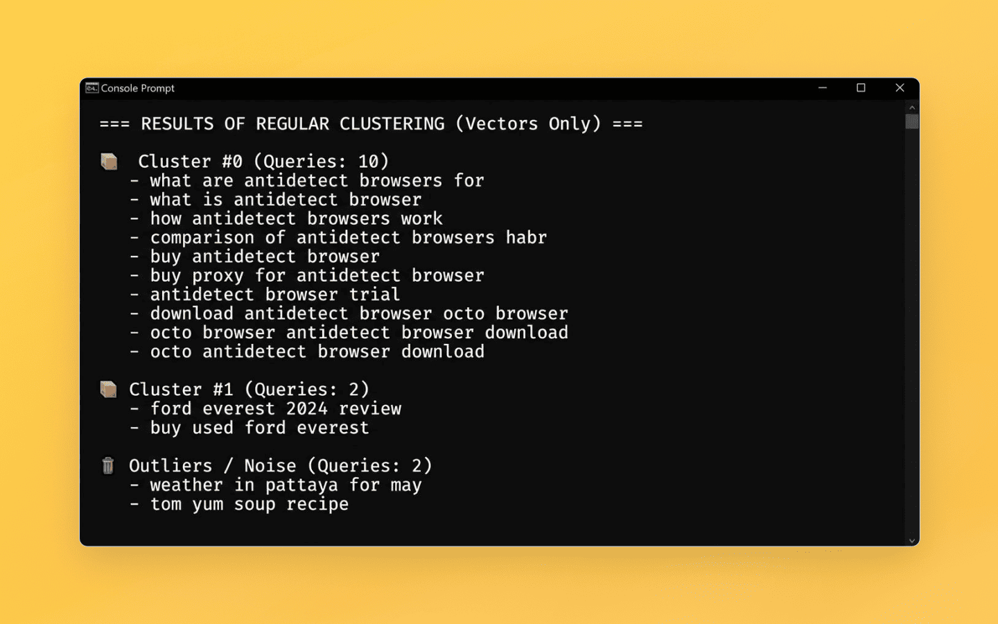
When clustering only by vector similarity, queries related to anti-detect browsers may end up in the same group despite differences in intent.

At this stage, the anti-detect browser once again becomes part of the pipeline, but not for collecting semantic data. Instead, it is used to collect SERP data. For each query, you need to collect search results and then use URL overlaps as an additional clustering signal.

With a large number of queries, this collection can be conveniently distributed across isolated browser profiles, for example by using Octo Browser together with Playwright or Puppeteer.

Related article

Web scraping Google Search results: tutorial (2026)

For each query, collect the top 10 URLs from the search results. Then, before running DBSCAN, compare the results for semantically similar phrases. If two queries have no common URLs or their number is below a defined threshold, the distance between the corresponding vectors is artificially increased.

Thus, embeddings are used to find semantically similar queries, while the SERP analysis acts as an additional constraint and helps prevent phrases with different search intents from being merged.

After adding search-result data, the test dataset discussed earlier in the article is distributed differently:

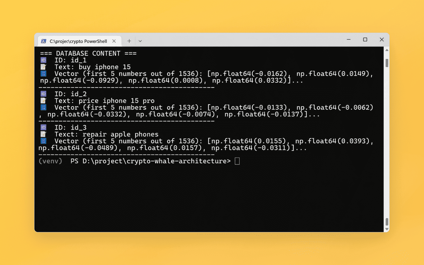
The number of clusters increases, and the groups themselves better match the intended search intent of the queries.

Post-processing results and updating data

After forming the clusters, there is one more practical task—assigning a clear name to each group. Numbers such as “Cluster #42” are convenient for an algorithm but tell an SEO specialist, editor, or content writer very little.

Automatic cluster naming with an LLM

When working manually, a specialist has to review the contents of each group, determine the primary intent, and come up with a name for the future page or piece of content. If there are several hundred clusters, this stage takes a significant amount of time.

This part of the process, however, can be automated with an LLM. The model receives a list of queries from one cluster, determines the overall intent, and generates an appropriate heading. You can use either cloud-based models or local solutions, e.g., Ollama.

It is important to define a strict output format in advance. If you simply ask the model to come up with a name, you may get additional explanations and comments along with the heading. That is why it is better to explicitly state in the system prompt that the output should contain only the heading with no additional text:

from openai import OpenAI

# 1. INITIALIZATION AND KEY
# Insert your actual API key here
client_ai = OpenAI(api_key="sk-YOUR_OPENAI_KEY")

# 2. OUR DATA (Result of hybrid clustering)
clusters = {
    0: [
       "what are anti-detect browsers for",
       "what is an anti-detect browser",
       "how anti-detect browsers work",
       "anti-detect browsers comparison",
    ],
    1: [
        "buy an anti-detect browser",
        "buy proxies for an anti-detect browser",
        "anti-detect browser trial"
    ],
    2: [
        "download anti-detect browser octo browser",
        "octo browser anti-detect browser download",
        "octo anti-detect browser download"
    ]
}

# System prompt (set rules for the model)
prompt = """You are an expert SEO specialist. Analyze the following cluster of search queries. Determine the primary user intent and generate one highly relevant H1 title for a future category page or article. Return ONLY the title, without any additional text, quotes or explanations."""

print("⏳ Sending clusters to GPT-4o-mini for automatic naming...\n")

# 3. Iterate through all clusters
for cluster_id, queries in clusters.items():
    # Send the queries from the current cluster to the API
    response = client_ai.chat.completions.create(
        model="gpt-4o-mini",
        messages=[
            {"role": "system", "content": prompt},
            {"role": "user", "content": "\n".join(queries)} # Combine the queries into a single text
        ],
        temperature=0.3
    )
    
    # Get the response
    h1_title = response.choices[0].message.content
    
    # Print the result to the console
    print(f"Cluster #{cluster_id}")
    print(f"Phrases: {', '.join(queries)}")
    print(f"Generated H1: {h1_title}\n")

from openai import OpenAI

# 1. INITIALIZATION AND KEY
# Insert your actual API key here
client_ai = OpenAI(api_key="sk-YOUR_OPENAI_KEY")

# 2. OUR DATA (Result of hybrid clustering)
clusters = {
    0: [
       "what are anti-detect browsers for",
       "what is an anti-detect browser",
       "how anti-detect browsers work",
       "anti-detect browsers comparison",
    ],
    1: [
        "buy an anti-detect browser",
        "buy proxies for an anti-detect browser",
        "anti-detect browser trial"
    ],
    2: [
        "download anti-detect browser octo browser",
        "octo browser anti-detect browser download",
        "octo anti-detect browser download"
    ]
}

# System prompt (set rules for the model)
prompt = """You are an expert SEO specialist. Analyze the following cluster of search queries. Determine the primary user intent and generate one highly relevant H1 title for a future category page or article. Return ONLY the title, without any additional text, quotes or explanations."""

print("⏳ Sending clusters to GPT-4o-mini for automatic naming...\n")

# 3. Iterate through all clusters
for cluster_id, queries in clusters.items():
    # Send the queries from the current cluster to the API
    response = client_ai.chat.completions.create(
        model="gpt-4o-mini",
        messages=[
            {"role": "system", "content": prompt},
            {"role": "user", "content": "\n".join(queries)} # Combine the queries into a single text
        ],
        temperature=0.3
    )
    
    # Get the response
    h1_title = response.choices[0].message.content
    
    # Print the result to the console
    print(f"Cluster #{cluster_id}")
    print(f"Phrases: {', '.join(queries)}")
    print(f"Generated H1: {h1_title}\n")

For the test dataset, the result might look like this:

Cluster #0
   Phrases: what are anti-detect browsers for, what is an anti-detect browser, how anti-detect browsers work
   Generated H1: What are anti-detect browsers used for

Cluster #1
   Phrases: buy an anti-detect browser, buy proxies for an anti-detect browser, anti-detect browser trial
   Generated H1: Best anti-detect browsers and proxies for safe browsing

Cluster #2
   Phrases: download anti-detect browser octo browser, octo browser anti-detect browser download, octo anti-detect browser download
   Generated H1: Download anti-detect browser Octo Browser

Cluster #0
   Phrases: what are anti-detect browsers for, what is an anti-detect browser, how anti-detect browsers work
   Generated H1: What are anti-detect browsers used for

Cluster #1
   Phrases: buy an anti-detect browser, buy proxies for an anti-detect browser, anti-detect browser trial
   Generated H1: Best anti-detect browsers and proxies for safe browsing

Cluster #2
   Phrases: download anti-detect browser octo browser, octo browser anti-detect browser download, octo anti-detect browser download
   Generated H1: Download anti-detect browser Octo Browser

In a real project, the number of clusters will be much larger, so storing the source data directly in the code is impractical. Usually, clusters are loaded from a file or database, and generated names are written back to the table for further work.

At this stage, the LLM is not involved in the clustering itself; it is used only to post-process already formed groups. This automates the routine part of the work and gives you a clear semantic-core structure without having to manually name every cluster.

Adding new queries

Another advantage of storing embeddings in ChromaDB is the ability to work with new data without manually performing a nearest-neighbor search across the entire dataset again.

After obtaining a new batch of semantic data, the queries go through the same pipeline: cleaning, vectorization, and adding them to ChromaDB. For each new embedding, you can find the nearest existing queries and evaluate the distance to them.

If the nearest neighbors belong to a stable existing cluster and meet the defined similarity threshold, the new query can be added to that group. If there is no suitable cluster, the query remains a candidate for forming a new group or is sent for additional processing.

This approach lets you use the accumulated vector database as an index for processing new queries and avoids performing a full pairwise search across the entire semantic core each time it is updated.

Conclusion

Building your own pipeline based on embedding models, vector storage, and clustering algorithms takes time, as you need to configure, test, and tune it. However, once this is done, you get a system that can be adapted to a specific topic, data volume, and project requirements.

The main advantages of this approach are:

• Reduced dependence on specialized services. You do not need a separate SEO service with fixed plans and volume limits for clustering. The main limitations shift to your own infrastructure: compute resources, memory, and disk space.

• Control over clustering logic. You can choose the embedding model yourself, configure eps, use SERP data, and change the rules for combining queries depending on the task.

• Control over the data. When using local models and local storage, semantic data remains within your own infrastructure and is not sent to third-party APIs.

The main value of this approach is not completely replacing ready-made SEO tools, but being able to build your own controllable pipeline. Use Octo Browser to automate semantic and SERP data scraping, and perform the rest of the processing locally with embeddings, ChromaDB, and clustering algorithms.

Once you build this process and carefully tune it using real data, it becomes more than a one-off script. It turns into a working tool that you can reuse and scale as your semantic core grows.